Additional implementations
This document is a supplement for unit 19, in which the numerical solution of ordinary differential equations (ODEs) was discussed in some details. In particular, there are two different implementations for the Forward Euler and Heun'method. For easy reference, the mathematical details of these methods are repeated below.
Use the codes provided below (or the ones in the original document) to answer questions 1, 2, 3 from Week 10.
If you have not yet covered ODEs in Calculus, please visit the link below where you are going to find information on first-order ODEs:
https://www.mathcentre.ac.uk/courses/mathematics/differential-equations/
Numerical approximations for IVPs
Numerical approximations of differential equations are based on replacing the continuous independent variable $x$ with a set of discrete points. This is referred to as a mesh or grid.
A mesh can be coarse or fine, depending on the number of points it contains.
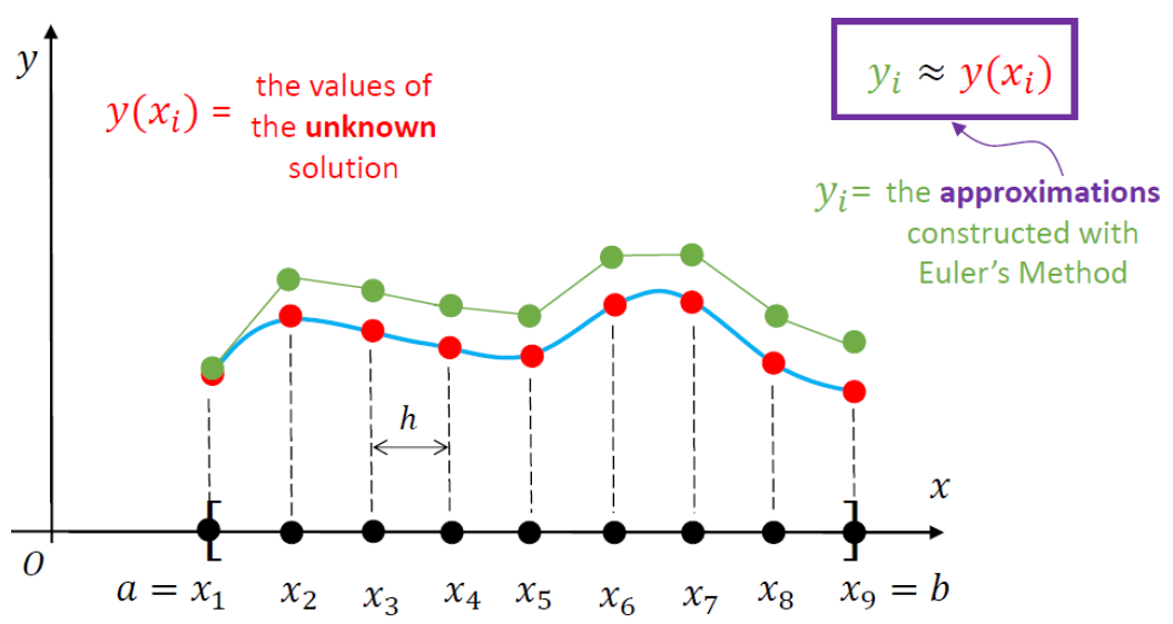
The goal of any numerical scheme for solving a given IVP consists in finding approximations for the
values of the unknown function $y(x)$ at the points of the mesh.
The sketch included below illustrates the notation associated with such a numerical approximation.
(Note that in Python we would start with $a=x_0$, then $x_1=x_0+h$, and so on -- so the sketch included below is slightly misleading because the first point in the mesh is $x_1$ rather than $x_0$.)
Forward Euler
This is the simplest numerical scheme for solving differential equations.
\begin{gather*}
y'(x) = f(x, y(x)),\qquad a\leq x \leq b\\
y(a) = y_0\quad\mbox{(given)}
\end{gather*}
The first step is to consider a uniform mesh over $[a,b]$,
$$
a = x_0 < x_1 < x_2 < ... < x_{n-1} < x_n = b\,,\qquad x_j = a + j h\,,
$$
where
$$
h = \frac{b-a}{n}\quad \mbox{(represents the mesh step size)}\,.
$$
The key idea in this solution strategy (F.E.) is to approximative the derivative
of our differential equation on the mesh. Before we examine that in detail, you
may recall that
$$
y'(x) = \lim_{\Delta x \to 0}\frac{y(x+\Delta x)-y(x)}{\Delta x}\quad\Longrightarrow\quad
y'(x)\simeq \frac{y(x+\Delta x)-y(x)}{\Delta x}\,,
$$
which is true if $|\Delta x|$ is very small (i.e., close to zero). With this in mind we can then write
$$
y(x+\Delta x) = y(x)+y'(x)\Delta x\,,\qquad\qquad\qquad\mbox{(4)}
$$
where I replaced "$\simeq$" with the equality sign "$=$".
In equation (4) we replace $x\to x_j$ and $\Delta x\to h$, to get
$$
y(x_j + h) = y(x_j) + hy'(x_j)\,.\qquad\qquad\qquad\mbox{(5)}
$$
If in the original differential equation we set $x\to x_j$, we obtain
$$
y'(x_j) = f(x_j, y(x_j))\,.\qquad\qquad\qquad\mbox{(6)}
$$
Combining (5) and (6) leads to
$$
y(x_j + h) = y(x_j) + h f(x_j, y(x_j))\,.
$$
Since $y(x_j + h) = y(x_{j+1})\simeq y_{j+1}$ and $y(x_j)\simeq y_j$, the last equation can be cast in the form
<font color = "Red"> $$ y_{j+1} = y_j + hf(x_j, y_j)\qquad\mbox{for}\quad j=0,1,2,\dots, (n-1)\qquad\qquad\qquad\mbox{(7)} $$ </font>
Equation (7) is a recurrence relation that represents the Forward Euler finite-difference scheme for finding a numerical approximation of the original initial-value problem.
This is how it works: we set $j=0$, then $j=1$, etc:
\begin{alignat*}{1}
&y_1 = y_0 + hf(x_0, y_0)\qquad (y_0\mbox{ is given; and so are $h$ and $f(x,y)$})\\[0.2cm]
&y_2 = y_1 + hf(x_1, y_1)\\[0.2cm]
&y_3 = y_2 + hf(x_2, y_2)\\[0.2cm]
&y_4 = y_3 + hf(x_3, y_3)\\[0.2cm]
&\dots \mbox{ ETC.}
\end{alignat*}
Numerical Implementation
# simple implementation of the forward euler numerical method:

from matplotlib import pyplot as plt
import numpy as np

#------------------------------------------------------------------------------
# this is the actual Euler solver:
def eulerFWD(fname, a, b, y0, N):

    # fname = name of the function that defines the RHS of your ODE
    # a, b  = left and right end points, respectively (a <= x <= b)
    # y0    = value of the solution at x = a; the initial condition is y(a) = y0
    # N     = there will be N sub-intervals in the mesh chose; note that this is directly
    #         related to the meshsize 'h'

    h = (b-a)/N                  # meshsize
    x = a + np.arange(N+1)*h     # the mesh
    y = np.zeros(len(x))         # array for storing the approx. soln.
    y[0] = y0                    # you know the first element of y (from the IC)

    # this is the implementation of the calculations immediately above this code:
    for k in range (N):
        y[k+1] = y[k] + h*fname(x[k], y[k])
    return (x, y)

#------------------------------------------------------------------------------
# this is what I referred to as the "right-hand side" above:
def myf(x, y):
    return (6*x**2-1.0)*y       # y' = (6*x**2-1)*y,  y(0) = 1

#-------------------------------------------------------------------------------
# this is the demo function:
def main():
    y0 = 1                                    # see above
    Nlist = [2**k for k in range(2,6,3)]      # a list of values for N (using list comprehensions)
    for N in Nlist:
        (x, y) = eulerFWD(myf, 0, 1, y0, N)
        plt.plot(x, y, 'b', x, y, 'ro')

    plt.xlabel('x')
    plt.ylabel('y')
    plt.grid(True)
    plt.show()
main()

Heun's Method (numerical implementation)
This is a predictor-corrector method, which means that the approximation at each step involves a two-stage process:
PREDICTOR STEP:
$$ y_{i+1}^* = y_i + hf(x_i, y_i) $$
CORRECTOR STEP:
$$ y_{i+1} = y_i + \frac{h}{2}\left[f(x_{i+1}, y_{i+1}^*)+f(x_i, y_i)\right] $$
This is also a second-order method (so it is superior to the Forward Euler strategy, which is only a first-order method). Broadly speaking this means that for Heun:
$$ |y(x_i)-y_i| = \mathcal{O}(h^2)\,, $$
while for F.E.,
$$ |y(x_i) - y_i| = \mathcal{O}(h)\,. $$
In particular, this means that in the former case you won't have to consider a very small stepsize in order to obtain a decent approximation. You can find more on this method by following the link below:
# simple implementation of heun's method:

from matplotlib import pyplot as plt
import numpy as np

#------------------------------------------------------------------------------
def heun(fname, a, b, y0, N):

    # fname = name of the function that defines the RHS of your ODE
    # a, b  = left and right end points, respectively (a <= x <= b)
    # y0    = value of the solution at x = a; the initial condition is y(a) = y0
    # N     = there will be N sub-intervals in the mesh chose; note that this is directly
    #         related to the meshsize 'h'

    h = (b-a)/N                    # meshsize
    x = a + np.arange(N+1)*h       # the mesh
    y = np.zeros(len(x))           # array for storage
    y[0] = y0                      # ...since y(a) = y0 (this is exact)

    # tmp  -> predictor step
    # y[k+1] --> corrector step
    for k in range (N):
        tmp = y[k] + h*fname(x[k], y[k])
        y[k+1] = y[k] + 0.5*h*(fname(x[k+1], tmp) + fname(x[k], y[k]))
    return (x, y)

#-------------------------------------------------------------------------------
# this function defines the RHS of the ODE:
def myf(x, y):
    return (6*x**2-1.0)*y       # y' = (6*x**2-1)*y,   y(0) = 1

#--------------------------------------------------------------------------------
# demo code -- exactly as before (in the FE example):
def main():
    y0 = 1
    Nlist = [2**k for k in range(3,5)]     # controls the size of the mesh
                                           # change the values in 'range' to get other cases
    for N in Nlist:
        (x, y) = heun(myf, 0, 1, y0, N)
        plt.plot(x, y, 'b', x, y, 'ro')

    plt.xlabel('x')
    plt.ylabel('y')
    plt.grid(True)
    plt.show()
main()
