19 Numerical solutions of ODEs
In this session we are going to discuss some simple numerical strategies for finding the solution of a given first-order ordinary differential equation (ODE for short).
If you have not yet covered this topic in Calculus, please visit the link below where you are going to find information on first-order ODEs:
https://www.mathcentre.ac.uk/courses/mathematics/differential-equations/
19.1 Initial-Value Problems
An initial-value problem consists of an ODE together with an initial condition.
The ODE is typically of the form:
$$
\frac{dy}{dx} = f(x, y)\,.\qquad\qquad\qquad \mbox{(1)}
$$
In this equation $f(x, y)$ is a given function of two variables, while $y=y(x)$ is the unknown function that depends on $x$. Note that equation (1) can also be cast in the longer form
$$
y'(x) = f(x, y(x))
$$
where we are now using the dash-notation to indicate the derivative of $y$ with respect to $x$.
Solving such a differential equation amounts to finding an expression for the unknown function. It is possible to solve such ODEs with pen and paper only in a limited number of cases; separable ODEs can be solved in closed form, while linear ODEs can be reduced to a separable one by using an appropriate integrating factor.
Examples:
1).
$$
\frac{dy}{dx} = 1+y^2\quad\Longrightarrow\quad \frac{dy}{1+y^2}=dx\quad \mbox{(separable)}
$$
2).
$$
\frac{dy}{dx} = x+y\quad\Longrightarrow\quad \frac{dy}{dx}-y = x\quad\mbox{(linear)}
$$
3).
$$
\frac{dy}{dx} = x^2+y^3\quad \mbox{(no analytic solution)}
$$
In these examples the right-hand side corresponds to the obvious functions:
- Ex. 1: $f(x,y) = 1+y^2$.
- Ex. 2: $f(x,y) = x+y$.
- Ex. 3: $f(x,y) = x^2+y^3$.
The solution of a first-order ODE will always depend on one arbitrary constant. Hence, the equations mentioned above do not have just one solution, but an entire family of solutions.
EXAMPLE:
Take the equation in Ex. 2 above. It's a linear equation that is readily solved to give
$$
y(x) = -x - 1 + C e^x \qquad\mbox{(for some constant $C\in\mathbb{R}$)}\,.\qquad\qquad\qquad\mbox{(2)}
$$
The constant $C$ is fixed by prescribing what the value of $y(x)$ must be at some point, $x_0$ (say). That is, we are usually interested in the solutions of an ODE that satisfy the additional condition
$$
y(x_0) = y_0\,,\qquad\qquad\qquad\mbox{(3)}
$$
where $x_0$ and $y_0$ are given numbers. This additional constraint is known as an initial condition.
Typically, if an initial condition like (3) is specified, we are interested in finding the values of the function $y(x)$ for $x>x_0$.
EXAMPLE:
If in Ex.2 above we want the solution that satisfies $y(0)=1$, we can use (3) to obtain $C=2$, so the solution of our initial-value problem will then be
$$
y(x) = -x - 1+2e^x\,.
$$
Note that this expression is a function of $x$ only.
"""
plot of the solution of the linear IVP from Ex.2 with the
initial condition y(0) = 1
"""
%matplotlib notebook
from matplotlib import pyplot as plt
import numpy as np

xmax = 7
x1 = np.linspace(0, xmax, 1000)
x2 = np.linspace(0, xmax, 6)
y1 = -x1 - 1 + 2*np.exp(x1)
y2 = -x2 - 1 + 2*np.exp(x2)
plt.plot(x1,y1,'--b', x2, y2, '-or')
#plt.plot(x2,y2,'or')
plt.xlabel('x')
plt.ylabel('y')
plt.show()

19.3 Numerical approximations for IVPs
Numerical approximations of differential equations are based on replacing the continuous independent variable $x$ with a set of discrete points. This is referred to as a mesh or grid.
A mesh can be coarse or fine, depending on the number of points it contains.
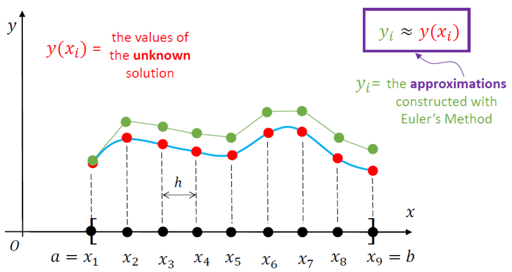
The goal of any numerical scheme for solving a given IVP consists in finding approximations for the
values of the unknown function $y(x)$ at the points of the mesh.
The sketch included below illustrates the notation associated with such a numerical approximation.
(Note that in Python we would start with $a=x_0$, then $x_1=x_0+h$, and so on.)
19.3.1 Forward Euler
This is the simplest numerical scheme for solving differential equations.
\begin{gather*}
y'(x) = f(x, y(x)),\qquad a\leq x \leq b\\
y(a) = y_0\quad\mbox{(given)}
\end{gather*}
The first step is to consider a uniform mesh over $[a,b]$,
$$
a = x_0 < x_1 < x_2 < ... < x_{n-1} < x_n = b\,,\qquad x_j = a + j h\,,
$$
where
$$
h = \frac{b-a}{n}\quad \mbox{(represents the mesh step size)}\,.
$$
The key idea in this solution strategy (F.E.) is to approximative the derivative
of our differential equation on the mesh. Before we examine that in detail, you
may recall that
$$
y'(x) = \lim_{\Delta x \to 0}\frac{y(x+\Delta x)-y(x)}{\Delta x}\quad\Longrightarrow\quad
y'(x)\simeq \frac{y(x+\Delta x)-y(x)}{\Delta x}\,,
$$
which is true if $|\Delta x|$ is very small (i.e., close to zero). With this in mind we can then write
$$
y(x+\Delta x) = y(x)+y'(x)\Delta x\,,\qquad\qquad\qquad\mbox{(4)}
$$
where I replaced "$\simeq$" with the equality sign "$=$".
In equation (4) we replace $x\to x_j$ and $\Delta x\to h$, to get
$$
y(x_j + h) = y(x_j) + hy'(x_j)\,.\qquad\qquad\qquad\mbox{(5)}
$$
If in the original differential equation we set $x\to x_j$, we obtain
$$
y'(x_j) = f(x_j, y(x_j))\,.\qquad\qquad\qquad\mbox{(6)}
$$
Combining (5) and (6) leads to
$$
y(x_j + h) = y(x_j) + h f(x_j, y(x_j))\,.
$$
Since $y(x_j + h) = y(x_{j+1})\simeq y_{j+1}$ and $y(x_j)\simeq y_j$, the last equation can be cast in the form
<font color = "Red"> $$ y_{j+1} = y_j + hf(x_j, y_j)\qquad\mbox{for}\quad j=0,1,2,\dots, (n-1)\qquad\qquad\qquad\mbox{(7)} $$ </font>
Equation (7) is a recurrence relation that represents the Forward Euler finite-difference scheme for finding a numerical approximation of the original initial-value problem.
This is how it works: we set $j=0$, then $j=1$, etc:
\begin{alignat*}{1}
&y_1 = y_0 + hf(x_0, y_0)\qquad (y_0\mbox{ is given; and so are $h$ and $f(x,y)$})\\[0.2cm]
&y_2 = y_1 + hf(x_1, y_1)\\[0.2cm]
&y_3 = y_2 + hf(x_2, y_2)\\[0.2cm]
&y_4 = y_3 + hf(x_3, y_3)\\[0.2cm]
&\dots \mbox{ ETC.}
\end{alignat*}
Numerical Implementation
INPUT:
* f(x, y) = RHS of the ODE.
* a, b    = endpoints of the x-range.
* n       = related to the number of points in the mesh.
Once you have the above you can go on and define h, as well as the mesh (which will have to be stored in a numpy array).
We can also specify h, as in the implementation below. Note that in this case the step size of the last step won't be the same as h.
OUTPUT:
* a numpy array containing the values of the approximations obtained by using
the above recurrence relation.import numpy as np
def solverFE(f, x, y, xstop, h):
'''Simple Forward Euler integrator '''
# initialise the storage for the solution:
xvals = []
yvals = []
#
# add the initial condition:
xvals.append(x)
yvals.append(y)
while x < xstop:
h = min(h, xstop - x)
y = y + h*f(x, y)
x = x + h
xvals.append(x)
yvals.append(y)
return np.array(xvals), np.array(yvals)
# note that this function returns 2 arrays, so you'll need to use 2 arrays
# to "catch" what the function returns
# A very simple check for the above function
# We are just plotting the solution that is computed
# Recall that this is Ex.2 above

%matplotlib notebook
from matplotlib import pyplot as plt

# This is the right-hand side of the ODE:
def f(x, y):
    return x + y

# Inputs:
xinit = 0
yinit = 1.0
xstop = 7.0
hs = 0.1

# Call the integrator
# Note that I am using two arrays to "catch" the returned output:
xvals, yvals = solverFE(f, xinit, yinit, xstop, hs)

# Plot the solution:
plt.plot(xvals,yvals,'--')
plt.xlabel('x')
plt.ylabel('y')
plt.show()

The above lines of code are simply used to check that our code runs smootly and produces some output that can be plotted as seen above. However, this is hardly a test of the accuracy of our code.
To test an initial-value solver we have several options:
- If an analytical solution is available, we can check the numerically computed approximation against the exact solution. This comparison can be in the form of a plot that contains both sets of data, although such an approach fails to give us a precise indication of the absolute and relative errors (A.E. and R.E., respectively).
- If an analytical solution is not readily available we can explore what happens if *h* (the stepsize) is decreased -- in principle, both A.E. and R.E. must go down.
# A very simple TEST for the above function
# We are running the code with 4 different values of h
# and then plot the solutions
# Recall that this is Ex.2 above

%matplotlib notebook
from matplotlib import pyplot as plt

# This is the right-hand side of the ODE:
def f(x, y):
    return x + y

# Inputs:
xinit = 0
yinit = 1.0
xstop = 3.0
hvals = [0.5, 0.05, 0.001, 0.0001]  #stepsize values used

# Initialize lists for storing the numerical results:
xvals = []
yvals = []
# Call the integrator (Forward Euler):
for h in hvals:
    xval, yval = solverFE(f, xinit, yinit, xstop, h)
    xvals.append(xval)
    yvals.append(yval)

# Plot the solutions obtained
# The last two curves overlap -- you must zoom in
#                    to convince yourself of this...
mystring = ''
lines = []
labels = []
for i in range(4):
    # Plot the solution:
    lin, = plt.plot(xvals[i],yvals[i],'--')
    lines.append(lin)
    mystring = 'Stepsize: ' + str(hvals[i])
    labels.append(mystring)

plt.legend(lines, labels)
plt.xlabel('x')
plt.ylabel('y')
plt.show()

Recall that we have the analytical solution for this test problem, so we can actually compute the A.E. and R.E. for different meshes. The code included below uses the same four stepsize values as above, but we produce plots for A.E. and R.E., as explained in the comments.
# A simple TEST for the above solver function
# We are running the code with 4 different values of h,
# compute the A.E. and R.E. based on the EXACT SOLUTION
# (which happens to be available in this case), and then
# plot this using matplotlib.
# Recall that this is Ex.2 above

%matplotlib notebook
from matplotlib import pyplot as plt

# This is the right-hand side of the ODE:
def f(x, y):
    return x + y

# Write a function to evaluate the exact solution:
def y_exact(x):
    return -x-1 + 2*np.exp(x)

# Inputs:
xinit = 0
yinit = 1.0
xstop = 3.0
hvals = [0.5, 0.05, 0.001, 0.0001]  #stepsize values used


# Initialize lists for storing the numerical results:
xvals = []
AEvals = []
REvals = []
# Call the integrator (Forward Euler):
for h in hvals:
    xval, yval = solverFE(f, xinit, yinit, xstop, h)
    xvals.append(xval)
    ytmp = y_exact(xval)
    # Compute A.E. and R.E. and store them:
    absval = np.abs(yval - ytmp)
    relval = np.true_divide(absval, np.abs(ytmp))
    AEvals.append(absval)
    REvals.append(relval)

fig, axs = plt.subplots(1,2) # defines two windows placed on the same row
fig.tight_layout(pad=5)
fig.suptitle('Absolute and Relative error for Forward Euler')
for j in range(2,4):
    axs[0].plot(xvals[j], AEvals[j], label='h='+str(hvals[j]))  # left window
    axs[1].plot(xvals[j], REvals[j], label='h='+str(hvals[j]))  # right window

#for ax in axs.flat:
#    print(ax)
axs[0].set(xlabel='x', ylabel= 'A.E.')#; axs[0].axis('square')
axs[1].set(xlabel='x', ylabel= 'R.E.')#; axs[1].axis('square')

# add some legends:
axs[0].legend()
axs[1].legend()

axs[0].grid(True)
axs[1].grid(True)

plt.show()

19.3.2 Heun's Method
This is a predictor-corrector method, which means that the approximation at each step involves a two-stage process:
PREDICTOR STEP:
$$ y_{i+1}^* = y_i + hf(x_i, y_i) $$
CORRECTOR STEP:
$$ y_{i+1} = y_i + \frac{h}{2}\left[f(x_{i+1}, y_{i+1}^*)+f(x_i, y_i)\right] $$
This is also a second-order method (so it is superior to the Forward Euler strategy, which is only a first-order method). Broadly speaking this means that for Heun:
$$ |y(x_i)-y_i| = \mathcal{O}(h^2)\,, $$
while for F.E.,
$$ |y(x_i) - y_i| = \mathcal{O}(h)\,. $$
In particular, this means that in the former case you won't have to consider a very small stepsize in order to obtain a decent approximation. You can find more on this method by following the link below:
#
# Numerical implementation of Heun's method
#
import numpy as np

def solverHEUN(f, x, y, b, h):
    # Create empty lists to store the x and y-values:
    X = []
    Y = []
    # Before the iteration starts, add x0 and y0 to the lists:
    X.append(x)
    Y.append(y)
    # Here starts the main iteration.
    # At each step the stepsize used will be h,
    #  except when we come to the end of the iteration.
    while x < b:
        h = min(h, b-x)
        ystar = y + h*f(x, y)
        y = y + 0.5*h*(f(x+h, ystar) + f(x, y))
        x = x + h
        X.append(x)
        Y.append(y)
    return np.array(X), np.array(Y)
# A very simple check for the HEUN solver
# We are just plotting the solution that is computed
# and compare it against the exact solution.
# Recall that this is Ex.2 at the top of this notebook

#%matplotlib notebook
from matplotlib import pyplot as plt
import numpy as np

# This is the right-hand side of the ODE:
def f(x, y):
    return x + y

# Inputs:
xinit = 0
yinit = 1.0
xstop = 7.0
hs = 0.1       # relativelyt large stepsize

# Call the HEUN integrator:
xvals, yvals = solverHEUN(f, xinit, yinit, xstop, hs)
y_exact = -xvals - 1.0 + 2.0*np.exp(xvals)  # exact solution

# Plot both the approximation and the exact solutions:
plt.plot(xvals[::5],yvals[::5],'or', label='NUMERICAL')
plt.plot(xvals, y_exact,'-b', label='EXACT')
plt.xlabel('x')
plt.ylabel('y')
plt.legend()
plt.show()
