20 Recursion
20.1 Recursive definitions
When the bisection method was introduced earlier in this module, there was an example of a game that required guessing a chosen number (the 'target') between 1 and 100, provided that we got some clues informing us whether our guess was either "high" or "low".
In the example seen previously (and included here for easy reference) the chosen number was 58; the strategy for guessing the number is outlined below:

The strategy of guessing the number above is a particular case of what computer scientists refer to as binary search. Initially, the range to search is the entire list of numbers (from 1 to 100). Our first step is to look at the middle item in the list. Should that turn out to be the target we are looking for, then we are finished. If it is not the target, we continue by performing binary search on either the top half or the bottom half of the list.
We can represent this in the form of specific algorithm.
Assume that we are searching for $x$ in a list of numbers: v[1] < v[2] < ..... < v[N].
# a version of the binary search algorithm (PSEUDOCODE):
# we have assumed that the numbers are placed in increasing order

# set the lower and upper bounds for the number to be guessed:
# (these will change as a result of the recursive calls)
vmin := v[1]
vmax := v[N]

# first guess:
mid := (vmin + vmax)//2                # note the integer division (remainder=discarded)
guess := mid

if mid == x:
    print('Number found', mid)         # this is the 'base case' (mentioned below)
    return
elif x < guess:
    perform binary search for x in [vmin,..., guess]
else:
    perform binary search for x in [guess, ..., vmax]
Note that instead of using a 'for-loop', this algorithm seems to refer to itself..... Furthermore, 'vmin' and 'vmax' will keep changing as the binary search function calls itself.
A description of something that refers to itself is called a recursive definition. In the above example, the binary search algorithm makes use of its own description. In other words, a call to binary search "recurs" inside of the definition -- hence, the label recursive definition.
Here's the Python implementation (using recursion) of the guessing game shown above:
# binary search using recursion

n = int(input('Give a number between 1 and 100: '))

def bsearch(val_min, val_max):
    mid = (val_min + val_max)//2

    guess = int(input('Give guess: '))

    if guess == n:
        print('\nThe number is: ', guess)
        return
    elif guess > n:
        print('\n***High***')
        print('The number is between ', val_min, ' and ', guess)
        val_max = guess
        bsearch(val_min, val_max)    # note that the function calls itself....
    else:
        print('\n*** Low ***')
        print('The number is between ', guess, ' and ', val_max)
        val_min = guess
        bsearch(val_min, val_max)    # the function calls itself again....
    return

# the external call of the 'bsearch()' function requires that
# the values passed to the 1st and 2nd parameters are the smallest and
# the largest numbers in our data set, respectively:

bsearch(1, 100)

# (those values are going to be changed during the internal calls)
In Mathematics there are many examples of recursive definitions. The classic one is the definition of the factorial:
$$ n! = n(n-1)(n-2)\dots(1) $$
For example $5! = 5(4)(3)(2)(1)$. If we remove the $5$ from the front, what remains is $4!$. In general, $n!=n(n-1)!$. We can therefore define the factorial recursively by setting
$$ n! = \begin{cases} 1\qquad &\mbox{if }n=0\\ n(n-1)! &\mbox{if }n\geq{1} \end{cases} $$
This definition says that the factorial of $0$ is (by definition) equal to $1$, while the factorial of any other number is defined to be that number times the factorial of one less than that number.
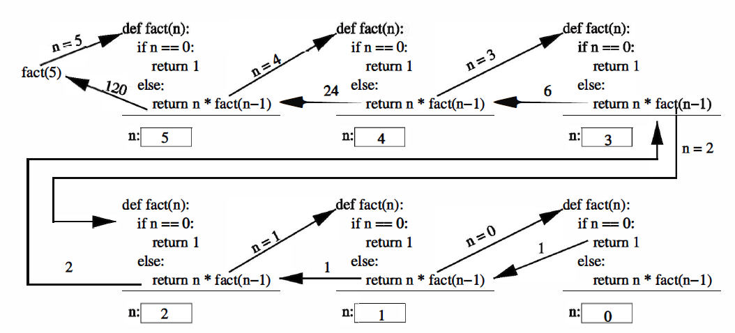
This definition is not circular because each application causes us to request the factorial of a smaller number. Eventually, the process will reach $n=0$, which does not require another application of the definition. This is called a base case for the recursion. When we reach the base case, the recursion ends because Python does not have to call the function anymore.
All good recursive definitions have the following two characteristics:
- there are one or more base cases for which no further recursion is required;
- all chains of recursion eventually end up at one of the base cases.
The implementation of the factorial using recursion is included below:
def fact(n):
    if n == 0:
        return 1
    else:
        return n*fact(n-1)

fact(5)   # 1*2*3*4*5
#fact(6)
#fact(7)
#(fact(8))
20.2 Fast exponentiation
A less obvious example of recursion is provided by the exponentiation. We can compute $a^n$ for any positive integer $n$ by simply multiplying $a$ by itself $n$ times:
$$ a^n = a*a*\dots *a $$
This can be easily implemented by using a simple loop:
# naive implementation of exponentiation
# using a 'for-loop':

def pow_1(a, n):
    power = 1
    for i in range(n):
        power *= a
    return power

def main():
    print(pow_1(2,7))

main()
# there is nothing wrong with this approach
This is okay, but we don't need so many multiplications.
Let's say we want to compute $2^8 = (2^4)(2^4)$. If we first calculate $2^4$, we can just do one more multiplication to get $2^8$.
Note that $2^4=(2^2)(2^2)$ and of course $2^2 = (2)(2)$.
Putting these together, it follows that we only need three multiplications to find $2^8$.
It should be clear that if $n$ is an even positive integer, then
$$ a^n = (a^{n/2})(a^{n/2})\,. $$
For $n=9$ (odd positive integer), we have $2^9 = (2^4)(2^4)(2)$ -- so we have an extra multiplication at the end. Thus, in the general case of an odd positive integer:
$$ a^n = (a^{n//2})(a^{n//2})(a)\,. $$
We can take advantage of these observations to implement exponentiation -- recursive style:
def pow_2(a, n):
    # raises 'a' to the integral power 'n'
    if  n==0:
        return 1                      # this is the base case
    else:
        factor = pow_2(a, n//2)
        #print('factor')              # uncomment to see how many recursive calls are made
        if n%2 == 0:                  # 'n' is EVEN
            return factor*factor
        else:                         # 'n' is ODD
            return factor*factor*a

# test the function:
pow_2(2,30)
20.3 The Fibonacci Sequence
The Fibonacci numbers $f_n$ correspond to the following definition:
$$ f_n = f_{n-1} + f_{n-2}\,,\qquad f_0 = f_1 = 1. $$
To compute the next Fibonacci number, we always need to keep track of the previous two. We can use two variables 'curr' and 'prev', to keep track of these values.
We then need a loop that adds together 'curr' and 'prev'; this will provide the next value in the Fibonacci sequence.
At that point, the old value of 'curr' becomes the new value of 'prev'. The code is included below:
# non-recursive implementation of the Fibonacci sequence

def classic_fib(n):
    # returns the nth Fibonacci number

    # the first two terms in the sequence:
    curr = 1    # f0
    prev = 1    # f1

    # next terms in the sequence:
    for j in range(n-1):
        curr, prev = curr + prev, curr
    return curr

# short demo:
def main():
    N=6
    for k in range(N):
        print('k =  ', k, '   Fibonacci:  ', classic_fib(k))


main()
# recursive implementation of the Fibonacci sequence

import timeit    # this module allows us to see how long a calculation takes

#---------------------------------------------------------------------------------
def fib(n):
    if n < 2:
        return 1
    else:
        return fib(n-1) + fib(n-2)
#---------------------------------------------------------------------------------
def main():
    k=5                                 # if this number is large,
    print('k = ', k,                     # the code is very slow....
          '   Fibonacci: ', fib(k))
#EndOfMain
#----------------------------------------------------------------------------------

# save the time at this point:
# ('start_time' will contain that value)
start_time = timeit.default_timer()

# call the main function:
main()

# display the CPU time required by main() to execute:
# from the current time at this point subtract what you stored earlier:
print('Computation time = {}'.format(timeit.default_timer()-start_time))
The implementation of the above algorithm is extremely inefficient. While the standard implementation ('classic_fib' above) can compute instantaneously the Fibonacci coefficients even for $k=5000$, the recursive version becomes very slow around $k=30$ (and even slower for larger values).
The reason for the slow execution time of the recursive version of the above code is directly linked to the large number of duplicate function evaluations that have to be performed. The diagram included below shows all the computations carried out by Python in order to find the result for $k=6$: fib(4) is calculated 2 times, fib(3) is calculated 3 times, fib(2) is calculated 5 times, an so on.
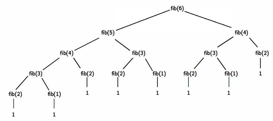
Key point: If you can solve a problem without using recursion, then use the other solution. Sometimes it might be very difficult to avoid using recursion. In those cases you need to ensure that the situation described above does not occur.
This does not mean that you have to give up on recursion. The next implementation still uses recursion, but at the same time we define a dictionary in which we are going to store the values that are calculated. Next time we need a specific term, instead of duplicating the computations, we are going to look up the stored value in the dictionary; this is a standard technique in computer science and is called memoization. Here is the relevant code:
# recursion --> improved version with memoization

import timeit

nval = 50             # index for the Fibonacci term
known = {0:1, 1:1}    # define a dictionary to store the values
                      # of the Fibonacci sequence
#--------------------------------------------------------------------------
def fibonacci(n):
    if n in known:        # looks for the key 'n' in the dictionary
        return known[n]   # returns the associated value, if it exists....

    # ... otherwise, use recursion:
    res = fibonacci(n-1) + fibonacci(n-2)
    known[n] = res                          # store the computed value
    return res                              # return the result as well

#---------------------------------------------------------------------------
def main():
    print('Fibonacci[{}] = {}'.\
           format(nval, fibonacci(nval)))

#EndOfMain
#----------------------------------------------------------------------------

# set the initial time:
start_time = timeit.default_timer()

# call the main function:
main()

# display the CPU time required by main() to execute:
print('Computation time = {}'.\
      format(timeit.default_timer()-start_time))
20.4 String reversal & anagrams
Some final examples. We are going to use recursion to compute the reverse of a string. That is, if the string is 'abc', we want the output to be 'cba'. One way to do this would be to use a list since Python lists come with a built-in method to reverse a list. However, on this occasion we are going to write our own implementation.
The basic idea is to think of a string as a recursive object. A string is made out of characters; we can think of a string as consisting of the first character plus a shorter string (or "the rest"). To reverse a string we reverse the shorter string and attach the first character on the end of that.
Say we want to reverse 'abcd'. This is 'a' + 'bcd'; we must reverse 'bcd' and then stick 'a' to the end of the reversed sub-string.
Take 'bcd', which is 'b' + 'cd'; we must reverse 'cd' and then stick 'b' to the end of the reversed sub-string.
Take 'cd', which is 'c' + 'd'; no need to reverse 'd', but we must stick 'c' after 'd' (that's the general rule in all the previous steps). This gives 'dc'. Going backwards, at the previous step we get 'dcb', and at the step before that (i.e., the first step above), we find 'dcba'. This is the reversed original string.
The implementation of the above recursive algorithm is included below (there is no restriction placed on the length of the string):
def reverse(s):
    if s == "":               # the 'empty' string (the base case)
        return s
    else:
        return reverse(s[1:]) + s[0]

# let's test this code:
reverse("COURSEWORK")
reverse("DogGod")
reverse("Madam")
# the last two strings are 'palindromes' = a sequence of characters
# that reads the same backward as forward
reverse("Betty bought a bit of bitter butter")
An anagram is formed by re-arranging the letters of a word. We use the same principle as above to write a recursive function that generates a list of all the possible anagrams of a string. Don't use the code below with very long strings; for a string of $N$ characters, there are N! anagrams (that's a large number even if $N=5$).
To illustrate the process, consider again a simple string, 'abc' (say). This consists of 'a' and 'bc'. Generating the list of all the anagrams of this second sub-string gives ['bc', 'cb']. To add back the first letter, we need to place it in all possible positions in each of these two anagrams of the original sub-string; this yields ['abc', 'bac', 'bca', 'acb', 'cab', 'cba']. The first three come from placing 'a' in every possible place in 'bc', and the second three come from doing the same with 'cb'.
# recursive implementation for generating all the ANAGRAMS
# of a given string:

def anagrams(s):
    if s == "":                       # this is the base case
        return [s]
    else:
        ans = []
        for w in anagrams(s[1:]):
            for pos in range(len(w)+1):
                ans.append(w[:pos] + s[0] + w[pos:])
        return ans

#test the function:
anagrams("dog")